



0 引言
波浪,作为海洋中重要的水动力现象,在从外海向近岸传播的过程中,会因海床地形、近岸水深等因素的变化发生折射、绕射、反射等物理现象,尤其当海床地形呈现周期性变化时,若地形间距为波浪波长一半的整数倍时,波浪与地形会发生共振,此时波浪反射最强,该现象被称之为波浪布拉格共振[1]。同时,波浪作为重要的海洋荷载,会对近海建筑物安全及海岸环境演变产生重要影响。珊瑚礁是海洋中最具生物多样性的生态系统之一,广泛分布于全球的热带和亚热带区域。 环礁[2]是常见的珊瑚礁类型,以独特的圆环形状和中央潟湖为典型特征,整体由礁坪环绕而成,外围发育出露海面的礁冠和陡峭的礁前斜坡。环礁通常发育一个或多个口门,用以连接潟湖与外海,对区域水动力环境和生态平衡具有重要调控作用。
目前,国内外学者已通过现场观测、物理模型实验和数值模拟等手段,针对珊瑚礁水动力相关问题开展了大量研究。在现场观测方面,HARDY等[3]在位于澳大利亚的约翰·布鲁尔礁进行现场实验,测量了短重力波穿过近海珊瑚礁时的衰减和变形情况;ROBERTS等[4]在大开曼岛的实地研究揭示了珊瑚礁结构对抵达岸线前的深海波浪特性的显著影响。在物理模型实验领域,YAO等[5-6]运用物理模型分析了破碎波类型、位置、宽度和破碎度等指标随礁坪水深和礁前斜坡坡度的变化以及珊瑚礁礁冠对波浪传播形态的影响;姚宇等[7]研究了珊瑚礁礁坪宽度变化对近岸波浪传播的影响。在数值模拟方面,FANG等[8]基于Boussinesq方程的激波捕捉模型,模拟了波浪在岸礁上的传播、 变形和破碎过程;FANG等[9]结合实验和雷诺平均 Navier-Stokes (RANS) 模型,研究了孤立波对礁坪上垂直墙的冲击过程,探讨了孤立波在礁坪上的传播、变形和破碎等特性;诸裕良等[10]运用非线性 Boussinesq 方程数值软件 FUNWAVE-TVD,对礁坪上的波浪破碎过程与增水特征进行了数值模拟。
1 控制方程
针对线性波浪在珊瑚环礁地形上的反射和透射问题,构建了一个典型的二维地形模型,如图1所示。模型将整个海域划分为三个区域:区域1和区域3为水平海底,其水深分别为h1和h3;区域2为地形变化区,其水深表示为 h2=h(x),区域长度为d。
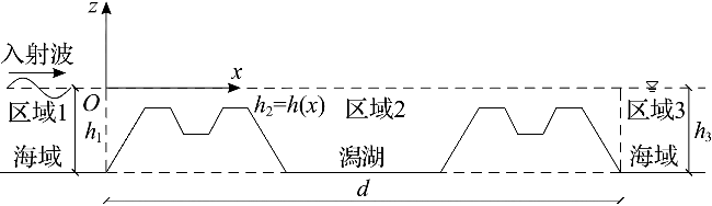
假设入射波振幅为A,圆频率为ω,根据线性波浪理论,可分别得到3个区域的速度势。在区域1,速度势ϕ(1)(x,z)可分解为入射势 ${\varphi }_{\mathrm{I}}^{\left(1\right)}$ (x,z)和反射势 ${\varphi }_{\mathrm{R}}^{\left(1\right)}$ (x,z):
ϕ(1)(x,z)= ${\varphi }_{\mathrm{I}}^{\left(1\right)}$ (x,z)+ ${\varphi }_{\mathrm{R}}^{\left(1\right)}$ (x,z)=- $\frac{\mathrm{i}gA}{\omega }$ ·(eikx+R0·e-ikx)· $\frac{\mathrm{c}\mathrm{o}\mathrm{s}\mathrm{h}k(z+{h}_{1})}{\mathrm{c}\mathrm{o}\mathrm{s}\mathrm{h}k{h}_{1}}$ =κ(1)(x)Z(1)(z)
式(1)中:i表示虚数单位,i= $\sqrt{-1}$ ;k为波数;g为重力加速度。
在区域2,应用修正缓坡方程,κ(2)(x) 满足[13]:
$ \begin{array}{c} \frac{\mathrm{d}}{\mathrm{~d} x}\left[c c_{\mathrm{g}} \frac{\mathrm{~d} \kappa^{(2)}(x)}{\mathrm{d} x}\right]+\left[k^{2} c c_{\mathrm{g}}+f_{1}\left(k h_{2}\right) g \frac{\mathrm{~d}^{2} h_{2}}{\mathrm{~d} x^{2}}+\right. \\ \left.f_{2}\left(k h_{2}\right) g k\left(\frac{\mathrm{~d} h_{2}}{\mathrm{~d} x}\right)^{2}\right] \kappa^{(2)}(x)=0 \end{array}$
式(2)中:c 和 cg 分别为波速和群速度;f1(kh2)和f2(kh2)分别为地形曲率项系数和坡度平方项系数,其均为kh2的函数[14]:
f1(kh2)= $\frac{-4k{h}_{2}\mathrm{c}\mathrm{o}\mathrm{s}k{h}_{2}+\mathrm{s}\mathrm{i}\mathrm{n}\mathrm{h}3k{h}_{2}+\mathrm{s}\mathrm{i}\mathrm{n}\mathrm{h}k{h}_{2}+8(k{h}_{2}{)}^{2}\mathrm{s}\mathrm{i}\mathrm{n}\mathrm{h}k{h}_{2}}{8\mathrm{c}\mathrm{o}\mathrm{s}{\mathrm{h}}^{3}k{h}_{2}·(2k{h}_{2}+\mathrm{s}\mathrm{i}\mathrm{n}\mathrm{h}2k{h}_{2})}$ - $\frac{k{h}_{2}}{2}$ $\frac{\mathrm{t}\mathrm{a}\mathrm{n}\mathrm{h}k{h}_{2}}{\mathrm{c}\mathrm{o}\mathrm{s}{\mathrm{h}}^{2}k{h}_{2}}$
f2(kh2)= $\frac{\mathrm{s}\mathrm{e}\mathrm{c}{\mathrm{h}}^{2}k{h}_{2}}{6(2k{h}_{2}+\mathrm{s}\mathrm{i}\mathrm{n}\mathrm{h}2k{h}_{2}{)}^{3}}$ · $\left[\begin{array}{l}8(k{h}_{2}{)}^{4}+16(k{h}_{2}{)}^{3}\mathrm{s}\mathrm{i}\mathrm{n}\mathrm{h}2k{h}_{2}-9\mathrm{s}\mathrm{i}\mathrm{n}{\mathrm{h}}^{2}2k{h}_{2}\mathrm{c}\mathrm{o}\mathrm{s}\mathrm{h}2k{h}_{2}+\\ 12\left(k{h}_{2}\right)(1+2\mathrm{s}\mathrm{i}\mathrm{n}{\mathrm{h}}^{4}k{h}_{2})(k{h}_{2}+\mathrm{s}\mathrm{i}\mathrm{n}\mathrm{h}2k{h}_{2})\end{array}\right]$
在区域3,速度势ϕ(3)(x,z)可表示为:
ϕ(3)(x,z)=- $\frac{\mathrm{i}gA}{\omega }$ ·T0·eikx· $\frac{\mathrm{c}\mathrm{o}\mathrm{s}\mathrm{h}k(z+{h}_{3})}{\mathrm{c}\mathrm{o}\mathrm{s}\mathrm{h}k{h}_{3}}$ =κ(3)(x)Z(3)(z)
式(1)~(5)中:R0和T0为待定系数;κ(j)(x)、Z(j)(z)、hj ( j=1, 2, 3) 分别为各区域中的待定函数、垂向特征函数、水深;k为波数,满足色散关系:
ω2=gktanhkhj (j=1, 2, 3)
相邻两区域交界面满足速度势连续和速度连续的匹配条件,具体参见式(7)~式(10)。
在区域1和区域2的交界面上 (x=0),匹配条件一为速度势连续:
κ(1)(x)=κ(2)(x) (x=0)
匹配条件二为速度连续:
同理,在区域2和区域3交界面上 (x=d) 也应有速度势连续:
κ(2)(x)=κ(3)(x) (x=d)
和速度连续:
应用中心差分格式对式(2)进行离散,整理可得:
$ \begin{array}{c} \left(\frac{c c_{\mathrm{g}}}{\Delta x^{2}}-\frac{\mathrm{d} c c_{\mathrm{g}}}{2 \mathrm{~d} x \Delta x}\right)_{i} \kappa_{i-1}^{(2)}+\left[k^{2} c c_{\mathrm{g}}+f_{1}\left(k h_{2}\right) \frac{\mathrm{d}^{2} h_{2}}{\mathrm{~d} x^{2}}+\right. \\ \left.f_{2}\left(k h_{2}\right)\left(\frac{\mathrm{d} h_{2}}{\mathrm{~d} x}\right)^{2}-\frac{2 c c_{\mathrm{g}}}{\Delta x^{2}}\right]_{i} \kappa_{i}^{(2)}+\left(\frac{c c_{\mathrm{g}}}{\Delta x^{2}}+\frac{\mathrm{d} c c_{\mathrm{g}}}{2 \mathrm{~d} x \Delta x}\right)_{i} \kappa_{i+1}^{(2)}=0 \\ (i=2,3, \cdots, n-1) \end{array}$
式(11)中:n 为节点总数;下标 i 为节点编号;Δx为空间离散步长,应满足每个波长上至少有8个节点[15]。
同样,对式(7)~式(10)进行离散可得:
-3 ${\kappa }_{1}^{\left(2\right)}$ +4 ${\kappa }_{2}^{\left(2\right)}$ - ${\kappa }_{3}^{\left(2\right)}$ + $\frac{2\mathrm{\Delta }xgAk}{\omega }$ ·R0= $\frac{2\mathrm{\Delta }xgAk}{\omega }$ (x=0)
综合式(11)~(15),可以得到n+2个线性方程,从而求得n+2个未知数( ${\kappa }_{1}^{\left(2\right)}$ , ${\kappa }_{2}^{\left(2\right)}$ ,…, ${\kappa }_{n}^{\left(2\right)}$ ,R0,T0),其中最后求得的待定系数R0即为反射系数KR,T0即为透射系数KT。
2 模型验证、数值实验设置与结果分析
2.1 模型验证
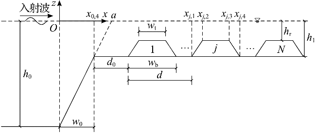
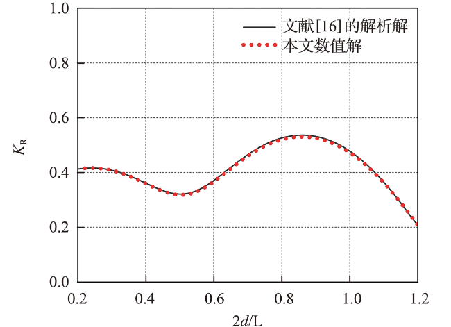
h(x)= $\left\{\begin{array}{ll}{h}_{0},& x\le 0\\ {h}_{0}-ax,& 0<x\le {x}_{\mathrm{0,4}}={w}_{0}\\ {h}_{1}-S(x-{x}_{j,1}),& {x}_{j,1}<x\le {x}_{j,2},j=1,\dots,N\\ {h}_{\mathrm{r}},& {x}_{j,2}<x\le {x}_{j,3},j=1,\dots,N\\ {h}_{\mathrm{r}}+S(x-{x}_{j,3}),& {x}_{j,3}<x\le {x}_{j,4},j=1,\dots,N\\ {h}_{1},& 其他\end{array}\right.$
式中:a=(h0-h1)/w0,代表礁前坡斜率;S=(h1-hr)/[(wb-wt)/2],代表梯形坝两侧的斜率。
2.2 数值实验设置
h(x)= $\left\{\begin{array}{ll}{h}_{0},& x\le {x}_{\mathrm{1,1}}=0\\ {h}_{0}-\mathrm{t}\mathrm{a}\mathrm{n}\theta ·x,& {x}_{\mathrm{1,1}}<x\le {x}_{\mathrm{1,2}}\\ {h}_{\mathrm{r}},& {x}_{\mathrm{1,2}}<x\le {x}_{\mathrm{1,3}}\\ {h}_{\mathrm{r}}+\mathrm{t}\mathrm{a}\mathrm{n}\beta ({h}_{0}-{h}_{\mathrm{r}})/\mathrm{t}\mathrm{a}\mathrm{n}\theta +\mathrm{t}\mathrm{a}\mathrm{n}\beta (x-{w}_{\mathrm{t}}),& {x}_{\mathrm{1,3}}<x\le {x}_{\mathrm{1,4}}\\ {h}_{1},& {x}_{\mathrm{1,4}}<x\le {x}_{\mathrm{2,1}}\\ {h}_{1}+\mathrm{t}\mathrm{a}\mathrm{n}\beta ({w}_{\mathrm{b}}+w-x),& {x}_{\mathrm{2,1}}<x\le {x}_{\mathrm{2,2}}\\ {h}_{\mathrm{r}},& {x}_{\mathrm{2,2}}<x\le {x}_{\mathrm{2,3}}\\ {h}_{0}+\mathrm{t}\mathrm{a}\mathrm{n}\theta (x-2{w}_{\mathrm{b}}-w),& {x}_{\mathrm{2,3}}<x\le {x}_{\mathrm{2,4}}\\ {h}_{0},& x>{x}_{\mathrm{2,4}}\end{array}\right.$
式中:h1为潟湖水深,h0为区域1和区域3的水深,hr为礁面到水面的垂直距离。
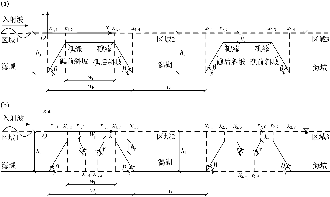
h(x)= $\left\{\begin{array}{ll}{h}_{0},& x\le {x}_{\mathrm{1,1}}=0\\ {h}_{0}-\mathrm{t}\mathrm{a}\mathrm{n}\theta ·x,& {x}_{\mathrm{1,1}}<x\le {x}_{\mathrm{1,2}}\\ {h}_{\mathrm{r}},& {x}_{\mathrm{1,2}}<x\le {x}_{\mathrm{1,3}}\\ {h}_{\mathrm{r}}+\mathrm{t}\mathrm{a}\mathrm{n}\gamma \left[x-({h}_{0}-{h}_{\mathrm{r}})/\mathrm{t}\mathrm{a}\mathrm{n}\theta -({w}_{\mathrm{t}}-{W}_{\mathrm{p}})/2\right],& {x}_{\mathrm{1,3}}<x\le {x}_{\mathrm{1,4}}\\ {h}_{\mathrm{r}}+{h}_{\mathrm{p}},& {x}_{\mathrm{1,4}}<x\le {x}_{\mathrm{1,5}}\\ {h}_{\mathrm{r}}+\mathrm{t}\mathrm{a}\mathrm{n}\gamma \left[({h}_{0}-{h}_{\mathrm{r}})/\mathrm{t}\mathrm{a}\mathrm{n}\theta +({w}_{\mathrm{t}}+{W}_{\mathrm{p}})/2-x\right],& {x}_{\mathrm{1,5}}<x\le {x}_{\mathrm{1,6}}\\ {h}_{\mathrm{r}},& {x}_{\mathrm{1,6}}<x\le {x}_{\mathrm{1,7}}\\ {h}_{\mathrm{r}}+\mathrm{t}\mathrm{a}\mathrm{n}\beta ({h}_{0}-{h}_{\mathrm{r}})/\mathrm{t}\mathrm{a}\mathrm{n}\theta +\mathrm{t}\mathrm{a}\mathrm{n}\beta (x-{w}_{\mathrm{t}}),& {x}_{\mathrm{1,7}}<x\le {x}_{\mathrm{1,8}}\\ {h}_{1},& {x}_{\mathrm{1,8}}<x\le {x}_{\mathrm{2,1}}\\ {h}_{0}-\mathrm{t}\mathrm{a}\mathrm{n}\beta (x-{w}_{\mathrm{b}}-w),& {x}_{\mathrm{2,1}}<x\le {x}_{\mathrm{2,2}}\\ {h}_{\mathrm{r}},& {x}_{\mathrm{2,2}}<x\le {x}_{\mathrm{2,3}}\\ {h}_{\mathrm{r}}+\mathrm{t}\mathrm{a}\mathrm{n}\gamma \left[x-{w}_{\mathrm{b}}-w-({h}_{0}-{h}_{\mathrm{r}})/\mathrm{t}\mathrm{a}\mathrm{n}\beta -({w}_{\mathrm{t}}-{W}_{\mathrm{p}})/2\right],& {x}_{\mathrm{2,3}}<x\le {x}_{\mathrm{2,4}}\\ {h}_{\mathrm{r}}+{h}_{\mathrm{p}},& {x}_{\mathrm{2,4}}<x\le {x}_{\mathrm{2,5}}\\ {h}_{\mathrm{r}}+\mathrm{t}\mathrm{a}\mathrm{n}\gamma \left[{w}_{\mathrm{b}}+w+({h}_{0}-{h}_{\mathrm{r}})/\mathrm{t}\mathrm{a}\mathrm{n}\beta +({w}_{\mathrm{t}}+{W}_{\mathrm{p}})/2-x\right],& {x}_{\mathrm{2,5}}<x\le {x}_{\mathrm{2,6}}\\ {h}_{\mathrm{r}},& {x}_{\mathrm{2,6}}<x\le {x}_{\mathrm{2,7}}\\ {h}_{\mathrm{r}}-\mathrm{t}\mathrm{a}\mathrm{n}\beta ({h}_{0}-{h}_{\mathrm{r}})/\mathrm{t}\mathrm{a}\mathrm{n}\theta +\mathrm{t}\mathrm{a}\mathrm{n}\beta (x-{w}_{\mathrm{t}}-{w}_{\mathrm{b}}-w),& {x}_{\mathrm{2,7}}<x\le {x}_{\mathrm{2,8}}\\ {h}_{1},& x>{x}_{\mathrm{2,8}}\end{array}\right.$
式中:h1为潟湖水深,h0为区域1和区域3的水深,hr为礁面至水面的距离。
2.3 潟湖相对深度对波浪反射及透射的影响
研究潟湖相对深度h1/h0对波浪反射系数KR和透射系数KT的影响,数值模型设置如图5所示。各参数取值如下:wb=7.6 m,wt=4 m,w=8 m,d=2wb+w,tanθ=1/6,tanβ=1/6,h0=0.35 m,hr=0.05 m,h1分别取0.15 m、0.175 m、0.25 m和0.35 m,对应的相对水深h1/h0分别为3/7、1/2、5/7和1。区域2的空间离散步长Δx=0.02 m,满足每个波长至少布置8个节点的要求[15]。入射波振幅A=0.01 m,波浪周期T从100.2 s减至7.2 s,对应波长L从185.6 m减至13.3 m,即2d/L从0.25增至3.50。
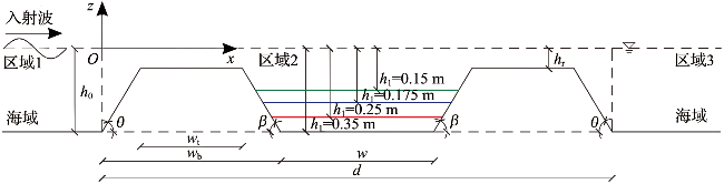
图6a展示了潟湖相对深度h1/h0变化下波浪反射系数KR的变化。随着h1/h0从3/7增加至1,波浪能量反射效率提升,共振时KR从0.900增加到0.956,对应的共振带的带宽逐渐变宽。随2d/L增加,不同工况下的KR均呈现出明显的周期性波动。当h1/h0=1时,在2d/L=0.965处,KR最高,达到了0.956,接近于1,表明波浪几乎被完全反射;当h1/h0=1/2和h1/h0=3/7时,KR则显著降低,在2d/L分别为0.849和0.824处,对应的KR峰值分别为0.916和0.900。
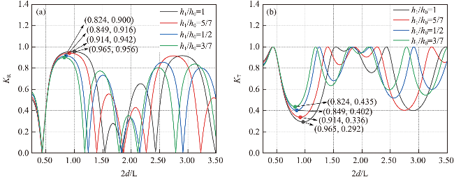
此外,随着潟湖深度的变化,波浪共振频率(即发生共振时反射及透射系数对应的2d/L所对应的波浪频率)也随之变化。具体从图6a中可以看到,随着h1/h0从3/7增加至1,共振峰向右偏移,峰值对应的2d/L从0.824逐渐增加至0.965。而经典布拉格定律预测共振会发生在2d/L=1处,本研究中的4种潟湖相对深度下,其2d/L均小于1,即共振频率相比经典布拉格定律发生了下移,随着潟湖相对深度的增加,频率下移的程度逐渐减小。究其原因,当潟湖水深较浅时,波浪的传播速度较慢,波浪若要产生布拉格共振反射需要更大的传播速度,而波长越长波浪传播速度越大,因此需要波长更长的波浪才能发生布拉格共振反射。故当水深较浅时,共振位置并不精确出现在2d/L=1处,而是在2d/L<1的位置。
图6b展示了潟湖相对深度h1/h0变化下波浪透射系数KT的变化。随着h1/h0的增加,波浪能量的透射效率降低,共振时透射系数从0.435减小到0.292;对应的共振带的带宽变宽;其谷值对应的2d/L从0.824逐渐增加至0.965,依旧均小于1,共振频率同样发生下移,随着潟湖相对深度的增加,频率下移程度逐渐减小。
2.4 采掘坑相对深度对波浪反射及透射的影响
研究采掘坑相对深度hp/h0对波浪反射系数KR和透射系数KT的影响,数值模型设置如图7所示。假设海底水平且不可渗透,h0=0.35 m,h1=0.35 m,hr=0.05 m。珊瑚环礁地形参数如下:wb=7.6 m,wt=4 m,w=8 m,tanθ=1/6,tanβ=1/6,tanγ=5/4,Wp=0.8 m。hp取0.05 m、0.15 m、0.25 m,对应的相对深度hp/h0分别为1/7、3/7、5/7。入射波振幅A=0.01 m,波浪周期T从100.2 s减至7.2 s,对应波长L从185.6 m减至13.3 m,即2d/L从0.25增至3.50。模型空间离散步长设置为Δx=0.02 m,满足每个波长至少布置8个节点的要求[15]。
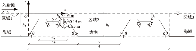
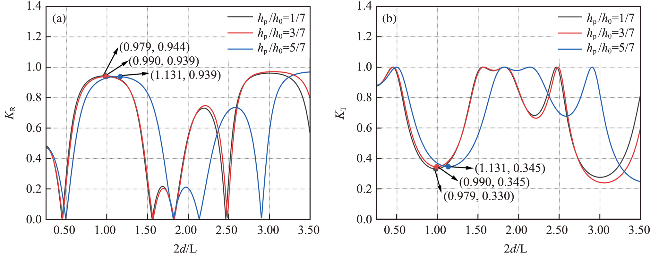
图8展示了采掘坑相对深度hp/h0变化下反射系数KR和透射系数KT的响应规律。随着 hp/h0从1/7增加至3/7,波浪发生共振时KR从0.944降至0.939(图8a); KT从0.330上升至0.345(图8b)。当 hp/h0从3/7增至5/7,共振时KR保持在0.939(图8a),而KT稳定在0.345(图8b)。这一结果表明,当hp/h0在3/7~5/7范围内,波浪共振时透射与反射达到了相对平衡状态。此外,对于反射及透射系数,当hp/h0=1/7和3/7时,其2d/L均小于1,波浪共振频率表现为下移;而随着hp/h0进一步从3/7增至5/7,共振位置对应的2d/L从0.990增加至1.131,此时2d/L大于1,即共振频率出现了明显的上移现象。


3 结论
本文基于修正缓坡方程有限差分模型,研究了珊瑚礁环礁地形中潟湖相对深度h1/h0和采掘坑相对深度hp/h0对波浪反射和透射的影响,计算并分析了波浪反射系数KR和透射系数KT的变化规律,主要结果如下。
1)随着潟湖相对深度h1/h0的增加,波浪发生布拉格共振时的反射系数显著提高,并且共振带的带宽也逐渐扩展。在较大的潟湖深度下,波浪几乎完全被反射,而较浅的潟湖则导致反射系数显著降低。波浪发生共振时对应的透射系数在潟湖相对深度增加过程中出现明显降低,表明波浪的能量传递效率下降。此外,在反射和透射过程中,波浪共振频率均发生下移,且下移程度随h1/h0增大而逐渐减小。
2)随着采掘坑相对深度hp/h0从1/7增加至3/7,波浪发生布拉格共振时的反射系数略有减小,透射系数则呈现一定的增加趋势;当hp/h0从3/7增加至5/7,波浪发生共振时的反射和透射系数保持稳定。同时,随着hp/h0由1/7至3/7,反射和透射时的共振位置对应的2d/L值均小于经典布拉格定律所预测的2d/L=1,其共振频率表现为下移;而随着hp/h0进一步增至5/7,共振位置对应的2d/L值均大于1,即波浪共振频率出现上移现象。
目前,有关波浪在珊瑚礁地形上传播的研究大多集中于单一因素的影响。例如,本文所提出的修正缓坡方程主要考虑了陡变地形因素,未考虑海床渗透等其他因素的影响。此外,波浪与海岸线的长期相互作用可能会导致地形演化。现有研究通常假设线性波浪条件,波浪的非线性作用、波浪的不规则性、底摩擦造成的能量损失、波浪破碎现象以及波流之间的相互作用等都未得到深入探讨,未来应关注这些方面,以更全面地理解波浪传播的复杂性。