
0 引言
1 模型介绍与改进方法
1.1 FVCOM数值模型
1.2 示踪物模块(DYE)
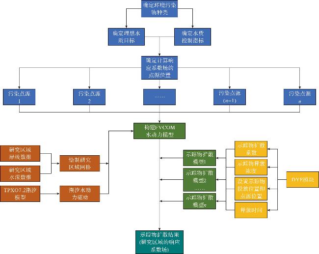
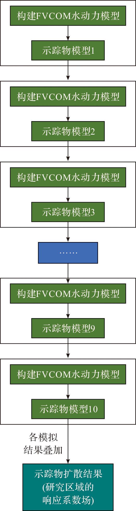
1.3 计算方法改进

2 模型配置与验证
表1 试验网格的主要参数设置Tab.1 Main parameter settings of the experiment grids |
| 试验名 | 三角元数 | 节点数 | 固边界 分辨率/km | 开边界 分辨率/km | |
|---|---|---|---|---|---|
| 理想矩形 网格 | 试验1 | 3 511 | 1 837 | 2.2 | 2.2 |
| 试验2 | 13 961 | 7 144 | 1.6 | 1.6 | |
| 试验3 | 55 326 | 27 984 | 1.1 | 1.1 | |
| 象山港岸线 网格 | 试验4 | 1 455 | 867 | 2.5 | 4.2 |
| 试验5 | 3 987 | 2 202 | 1.1 | 2.2 | |
| 试验6 | 15 065 | 8 045 | 0.5 | 1.0 | |
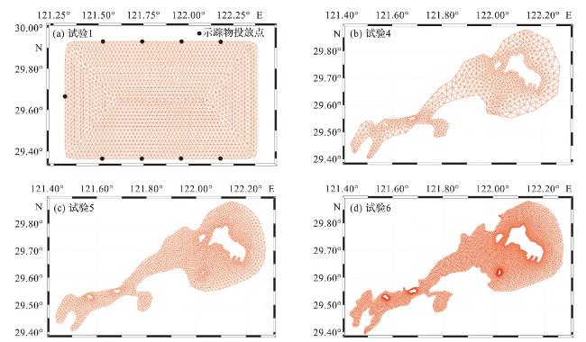
图4 试验网格图及理想矩形试验组示踪物投放点示意图(理想矩形试验2、3图略)Fig.4 Diagram of the grids and tracer release points for the ideal rectangular experiment group (figures for ideal rectangular experiments 2 and 3 are omitted) |

3 结果与讨论
3.1 流场模拟结果
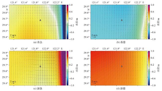
图6 理想矩形区域试验流场图(三角符号为判定落急、落憩、涨急和涨憩4个典型时刻的基准站。) Fig.6 Flow field of ideal rectangular experiment (The triangular symbol is the reference station for determining the four typical moments of ebb strength, ebb slack, flood strength and flood slack.) |

3.2 示踪物模拟结果
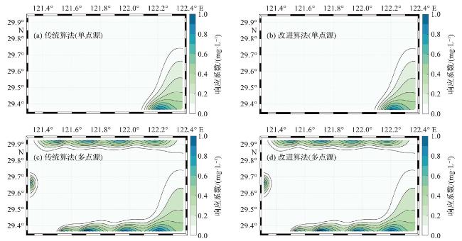
图8 理想矩形研究区中使用不同方法模拟单点源(a,b)和多点源(c,d)响应系数场(试验2)(改进算法和传统算法所得结果完全一致。) Fig.8 The response coefficient fields of single point source (a, b)and multiple point sources (c, d)in an ideal rectangular study area using different methods (experiment 2) (The results of improved algorithm case and original case are identical.) |
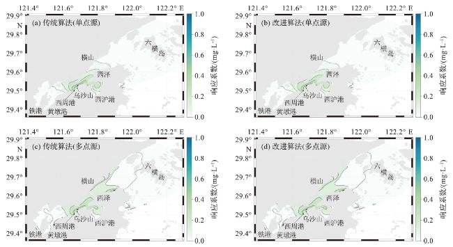
图9 象山港研究区中使用不同方法模拟单点源(a,b)和多点源(c,d)响应系数场(试验6)(改进算法和传统算法所得结果完全一致。) Fig.9 The response coefficient fields of single point source (a, b)and multiple point sources (c, d)in the Xiangshan Bay study area using different methods (experiment 6) (The results of improved algorithm case and original case are identical.) |
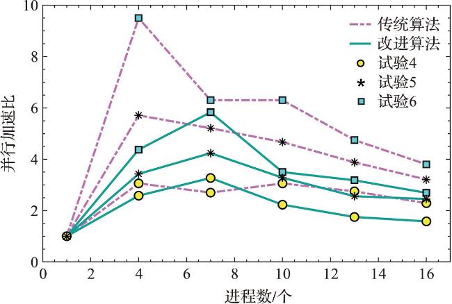
3.3 模型运行时间对比
表2 各试验模型运行时间对比Tab.2 Comparison of running time of experiments |
| 研究区 | 试验序号 | 模型运行时间/min | 运算速度 提升比 | |
|---|---|---|---|---|
| 传统算法 | 改进算法 | |||
| 理想矩形区域 | 试验1 | 3 627 | 557 | 85% |
| 试验2 | 9 054 | 2 370 | 74% | |
| 试验3 | 44 730 | 8 277 | 81% | |
| 象山港 | 试验4 | 95 | 35 | 63% |
| 试验5 | 137.5 | 49 | 64% | |
| 试验6 | 7 080 | 1 546 | 78% | |